About | Support | Discussion Forum | Index | Service Status | ros @ Robotics Stack Exchange

Obstacle Avoidance and Robot Footprint Model

Description: In this tutorial you will learn how obstacle avoidance is realized. Necessary parameter settings with a major focus on the robot footprint model and its influences are described.

Keywords: Trajectory Optimization Local Planner Navigation Obstacles Footprint

Tutorial Level: INTERMEDIATE

Next Tutorial: Following the Global Plan (Via-Points)

This tutorial targets version 0.3+ of the teb_local_planner package.

How Obstacle Avoidance works

Penalty terms

Obstacle avoidance is achieved as part of the overall trajectory optimization. Obviously, optimization is concerned with finding a minimum cost solution (trajectory) of a specified cost function (objective function). Put simply: If a planned (future) pose violates a desired separation from obstacles, the costs of the cost function must therefore increase. Ideally, the cost function value must be infinity in those cases or the optimizer might better reject those areas completely. However, this would require optimizers handling hard constraints (resp. solving nonlinear programs). The teb_local_planner waives the ability of taking hard constraints into account in order to better account for efficiency. Hard constraints are transformed into soft constraints, leading to the composition of quadratic penalty terms with finite costs.

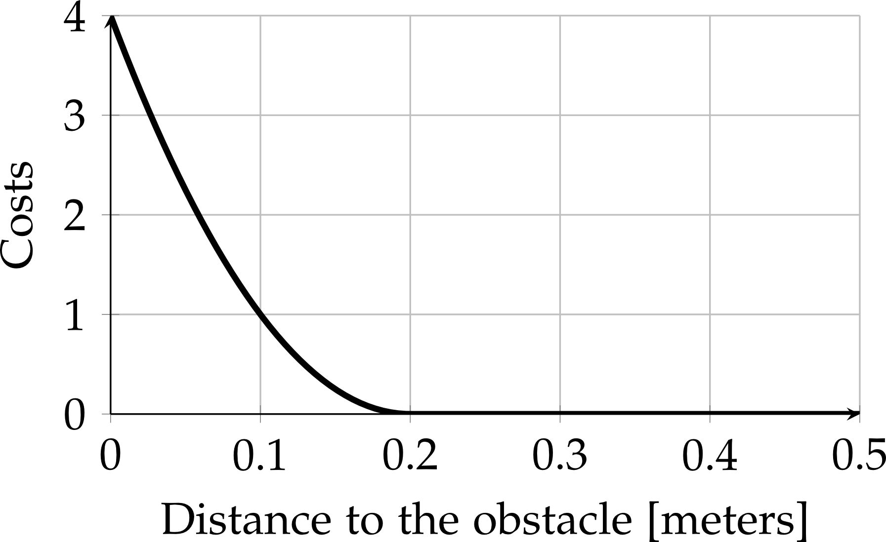
The figure above shows an examplary penalty term (for obstacle avoidance). The allowed minimum Euclidean distance to the obstacle (parameter min_obstacle_dist) is set to 0.2 meters. Therefore, distances below 0.2m lead to a non-zero cost. Now imagine that the optimization problem consists of many more cost terms. Some of them are conflicting such as time-optimality. Therefore it might happen, that the optimizer takes a small violation (and therefore small penalty) into account in order to minimize the overall composed cost function. Here you have two options in order to tune the behavior:

1. Adjust the optimization weights (scaling of the individual costs, here it is parameter weight_obstacle). But if you choose too high values, the optimization problem becomes ill-conditioned leading to a poor convergance behavior.

2. Shift the argument by adding an "extra margin". By adding a small extra margin to the min_obstacle_dist parameter you implicitly increase the cost value at 0.2m. You might shift all penalty terms at once with the single parameter penalty_epsilon, but be careful since doing so will massively influence the optimziation results.

Locally optimal solutions

Notice, the optimizer on its own only finds locally optimal solutions. Imagine, the robot might be encapsulated laterally by two obstacles. The penalty terms are indeed non-zero, but the optimizer get stucked (to this local minimum) since moving the corresponding pose laterally towards one of the obstacles would further increase the total cost. You can try that easily with the test_optim_node (see Tutorial Set up and test Optimization and turn off homotopy class planning). The behavior should be similar to the one in the following figure:

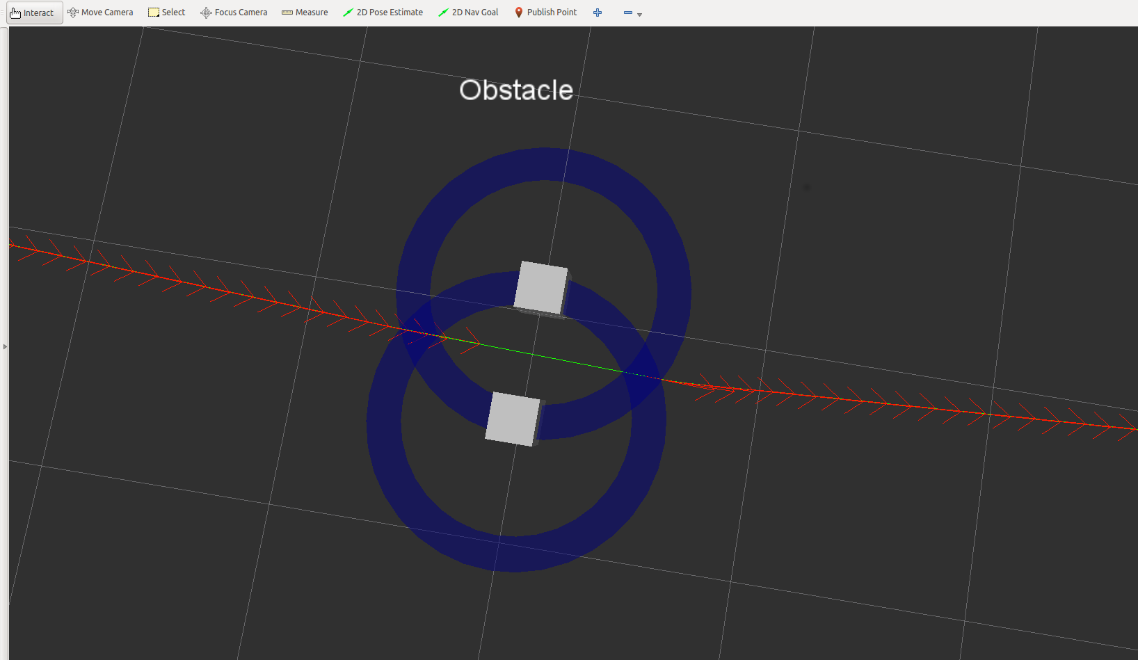
The trajectory cannot jump over the obstacles. Even the poses itselves are pushed away from the region between the obstacles (red arrows). Obviously, this circumstance should be avoided in practice. Hence, the homotopy class planning algorithm seeks for (topologically) alternative solutions and the feasibility check (see section below) rejects such a solution before actually commanding the robot.

Association between Poses and Obstacles

The following figure depicts a snapshot of a common planning scenario:

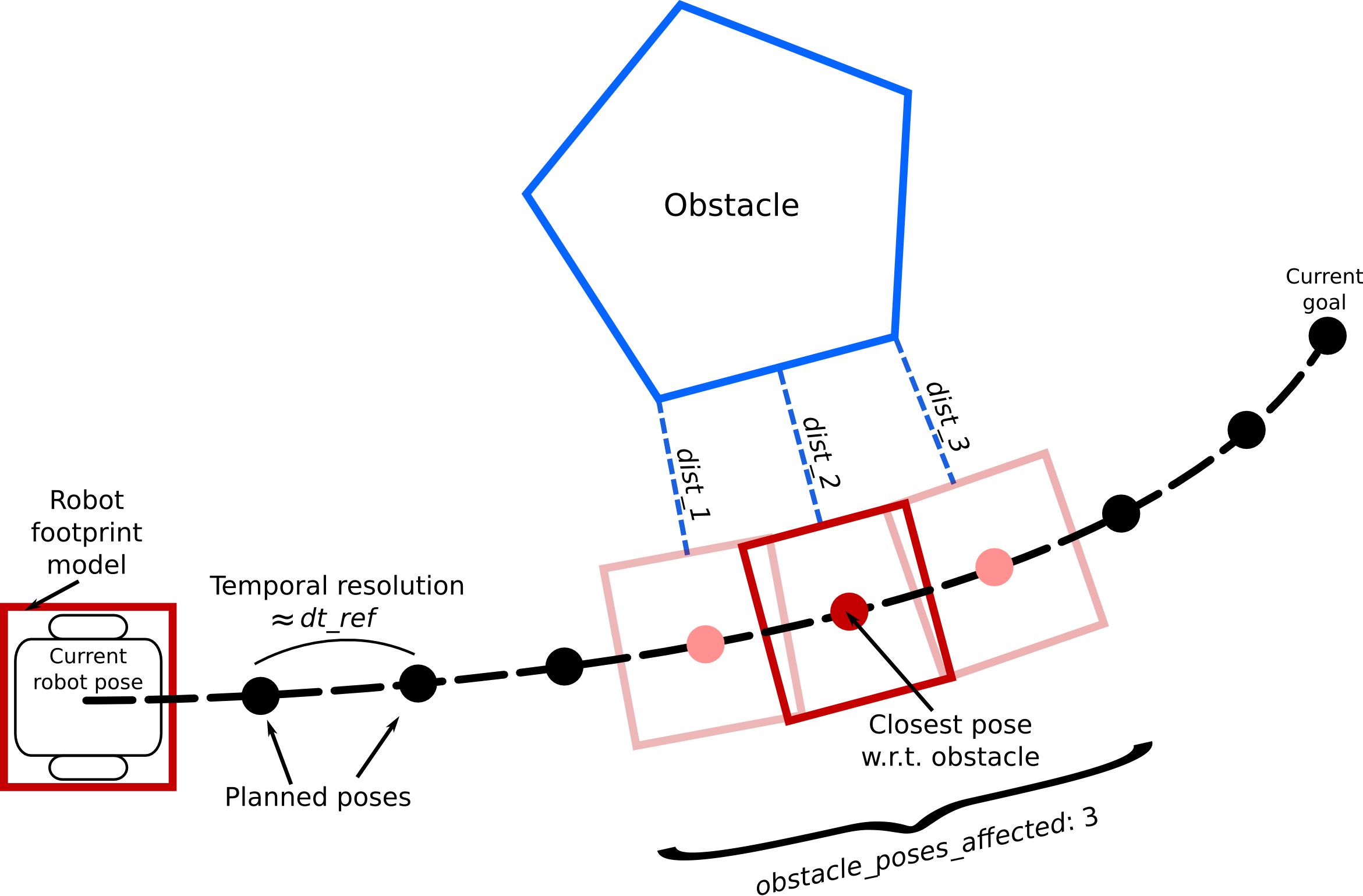
The scenario consists of a mobile robot which approaches a polygon-shaped obstacle while traveling to the current goal. The planned (discrete) trajectory is composed of multiple robot poses. The planner aims to arrange each two consecutive poses according to the desired temporal resolution (Parameter dt_ref). Note, the actual resolution is not fixed/freezed since the optimizer needs to adjust the transition time in order to seek for time-optimality.

For obstacle avoidance, the distance between a planned pose and the obstacle has to be bounded from below. The example trajectory in the figure consists of 8 changeable poses (start and goal poses are fixed). You might agree, that many distance calculations are required in order to achieve a collision free trajectory (the optimizer invokes the computation of cost function values many times). In order to speed up the optimization, a dedicated association strategy is implemented.

For each obstacle (point/ occupied costmap cell, line, polygon) the closest pose of the planned trajectory is located (see figure above). According to the value of parameter obstacle_poses_affected neighbors of the closest pose are taken into account as well. Only this selected subset of poses is taken into account in the subsequent optimization step (here 3 poses and therefore 3 penalty terms). The association process is repeated after no_inner_iterations (parameter), resp. within each outer optimization iteration. The value of obstacle_poses_affected slightly influences the smoothness of the trajectory around obstacles. Also bigger obstacles require more connected poses to avoid inadmissable shortcuts. You may also choose a high value (> trajectory length) in order to connect all poses with each obstacle.

Note, the robot footprint model is taken into account for distance calculations and is therefore crucial for the required computational resources. Details are summarized in the following section.

Robot Footprint Model

The robot footprint model approximates the robots' 2D contour for optimization purposes. The model is crucial for the complexity of distance calculations and hence for the computation time. Therefore, the robot footprint model constitutes a dedicated parameter instead of loading the footprint from the common costmap_2d parameters. The optimization footprint model might differ from the costmap footprint model (which is instead used for the feasibility check, see section below).

The footprint model is selected and configured using the parameter server. You can add the following parameter structure to your teb_local_planner config file:

TebLocalPlannerROS:
 footprint_model: # types: "point", "circular", "line", "two_circles", "polygon"
   type: "point"
   radius: 0.2 # for type "circular"
   line_start: [-0.3, 0.0] # for type "line"
   line_end: [0.3, 0.0] # for type "line"
   front_offset: 0.2 # for type "two_circles"
   front_radius: 0.2 # for type "two_circles"
   rear_offset: 0.2 # for type "two_circles"
   rear_radius: 0.2 # for type "two_circles"
   vertices: [ [0.25, -0.05], [0.18, -0.05], [0.18, -0.18], [-0.19, -0.18], [-0.25, 0], [-0.19, 0.18], [0.18, 0.18], [0.18, 0.05], [0.25, 0.05] ] # for type "polygon"

The default footprint model is of type "point".

Note, the footprint is published to ~<name>/teb_markers and can be visualized in rviz (e.g. for verification).

Important: For car-like robots, the pose [0,0] is located at the rear-axle (axis of rotation)!

All different types are described in the following paragraphs:

Footprint Type: Point

The robot is modeled as a single point. For this type the least computation time is required.

Footprint Type: Circular

The robot is modeled as a simple circle with a given radius ~/footprint_model/radius. The distance calculation is similar to the one of the point-type robot, but with the exepction, that the robots' radius is added to the parameter min_obstacle_dist each function call. You can ged rid of this extra addition by chosing a point-type robot and adding the radius to the minimum obstacle distance a-priori.

Footprint Type: Line

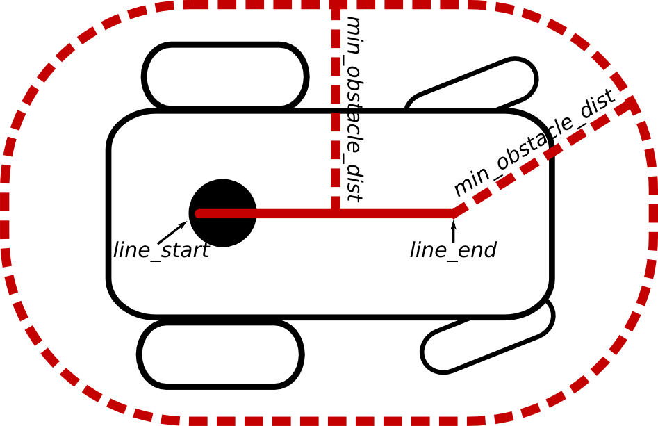
The line robot is useful for robots that exhibit different expansions/lengths in the longitudinal and lateral directions. The line (segment) can be configured using parameters ~/footprint_model/line_start and ~/footprint_model/line_end ([x,y] coordinates each). The robot (axis of rotation) is assumed to be at [0,0] (Unit: meters). Make sure to encapsulate the complete robot by further adjustment of the parameter min_obstacle_dist (see following example).

You might also have a look at the "two circles" model.

Footprint Type: Two Circles

Another possibility to approximate the robot's contour consists of defining two circles. Each circle is described by an offset along the robots' x-axis and a radius: ~/footprint_model/front_offset, ~/footprint_model/front_radius, ~/footprint_model/rear_offset and ~/footprint_model/rear_radius. Offsets may be negative.

Refer to the following figure as an example:

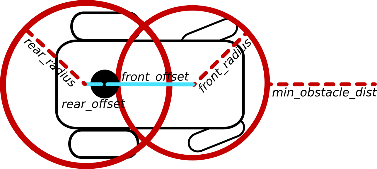
For each associated robot pose two distance calculations are necessary.

Footprint Type: Polygon

A complex model can be incorporated by defining a closed polygon. The polygon is defined in terms of a list of vertices (provide x and y coordinates for each vertex). The robots axis of rotation is assumed to be located at [0,0] (Unit: meters). Please do not repeat the first vertex since the polygon is closed automatically.

Take in mind, that each additional edge significantly increases the required computation time! You may copy your footprint model from your costmap common parameter file.

Feasibility Check

A feasibility check is performed after the optimizer returns a trajectory and before the velocity commands are sent to the robot. The purpose of this check is to identify an invalid/infeasible trajectory that might be produced by the optimizer (just remember: soft constraints, local minima, etc.).

Currently, the algorithm iterates the first n poses (n = ~/feasibility_check_no_poses (parameter!)) starting from the current robot pose and checks whether the those poses are collision free. For detecting if a collision occurs, the costmap footprint is used (see Navigation tutorials)! Therefore, this validation-model might be more complex than the footprint used for optimization (see section above).

The value ~/feasibility_check_no_poses should not be chosen too high, since the optimizer might not be converged completely: Figuratively, small obstacle violations in the (far) future could be corrected while the robot is moving towards the goal.

If you are driving in narrow environments, make sure to configure the obstacle avoidance behavior (local planner and global planner) properly. Otherwise, the local planner might reject an infeasible trajectory (from its point of view), but the global planner in contrast could further think that the selected (global) plan is feasible: the robot could get stucked.

Example Setup

You can find an example setup with the stage simulator in the teb_local_planner_tutorials package.

1. Install the teb_local_planner_tutorials package

2. Inspect and launch the carlike configuration